Preparation
Copy example data
file.copy(
  from = system.file('extdata', 'minimal', package = 'qntmap'),
  to = wd,
  recursive = TRUE
)
#> [1] TRUE
TRUE indicates copying is successful. Check copied files by dir().
dir(file.path(wd, 'minimal'), recursive = TRUE, all.files = TRUE)
#>  [1] ".map/1/0.cnd"        ".map/1/1_map.txt"    ".map/1/1.cnd"
#>  [4] ".map/1/2_map.txt"    ".map/1/2.cnd"        ".qnt/.cnd/elemw.cnd"
#>  [7] ".qnt/bgm.qnt"        ".qnt/bgp.qnt"        ".qnt/elem.qnt"
#> [10] ".qnt/elint.qnt"      ".qnt/mes.qnt"        ".qnt/net.qnt"
#> [13] ".qnt/pkint.qnt"      ".qnt/stg.qnt"        ".qnt/wt.qnt"
#> [16] "conditions_qnt.csv"  "conditions_xmap.csv" "README.md"
Analysis
Load data
# Read X-ray mapping data
xmap <- read_xmap(dir_map)
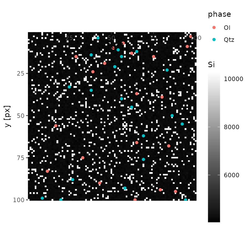
# Read spot analysis data
qnt <- read_qnt(dir_qnt, renew = TRUE)The example data contains olivine and quartz in the mapping area. The phases are quantified 20 points each.
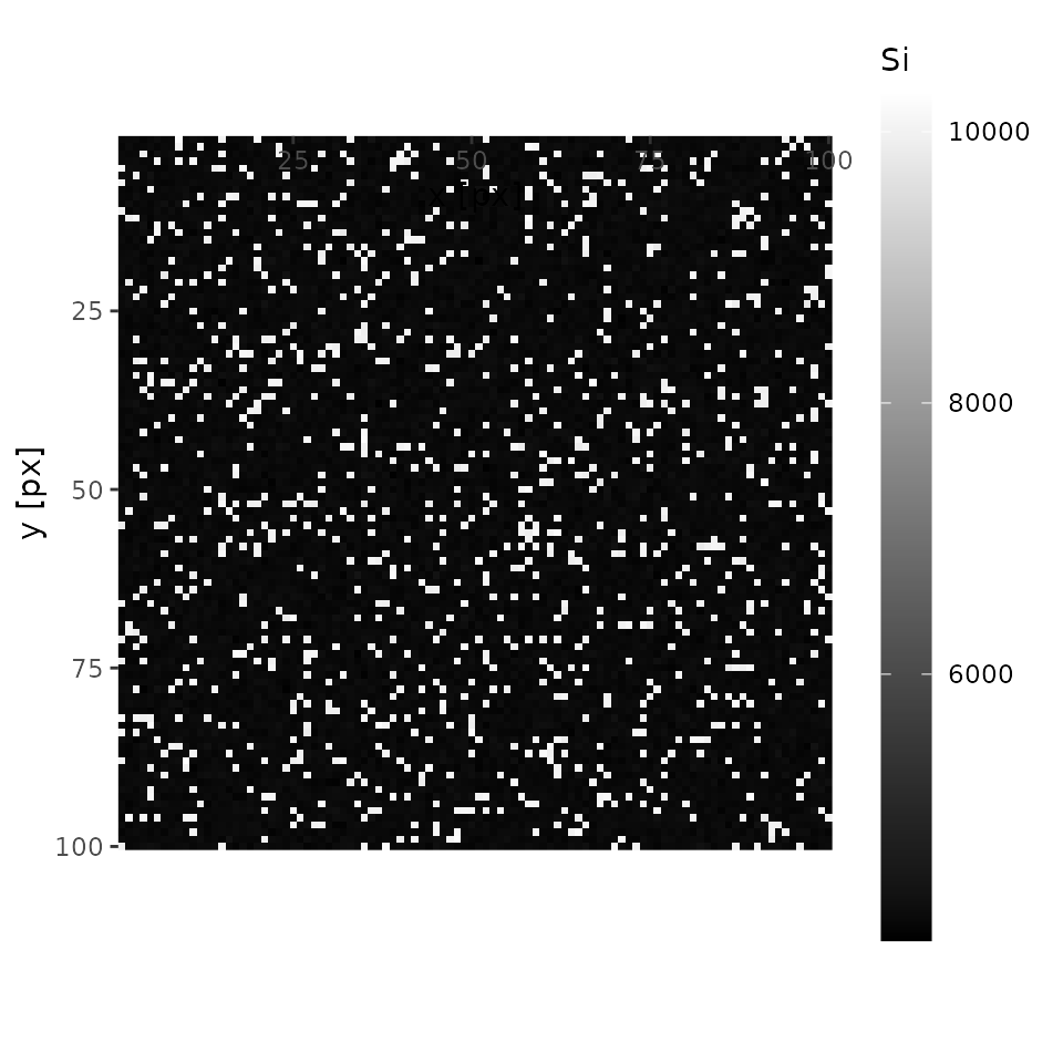
Plot X-ray maps
Plots are interactive with Web UI. Elements can be chosen by mouse actions.
plot(xmap)
# A following plot is non-interactive mode run by
# plot(xmap, 'Mg', interactive = FALSE)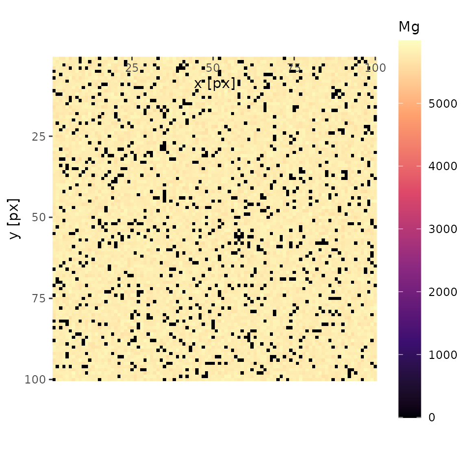
Cluster analysis
Initialize cluster centers
This step guesses initial cluster centers (i.e., mean mapping intensities of each phase). Check if results are adequate by comparing them with plots. If inadequate, consider modifying values
centers <- find_centers(xmap, qnt)
print(centers)
#>   phase      Si      Mg
#> 1    Ol  4263.8 5722.45
#> 2   Qtz 10002.0    0.00
Run cluster analysis
A result is saved as a binary file and PNG images in clustering directory below the directory containing mapping data.
For a quick look, plot() function is also available.
cluster <- cluster_xmap(xmap, centers)
plot(cluster, interactive = FALSE)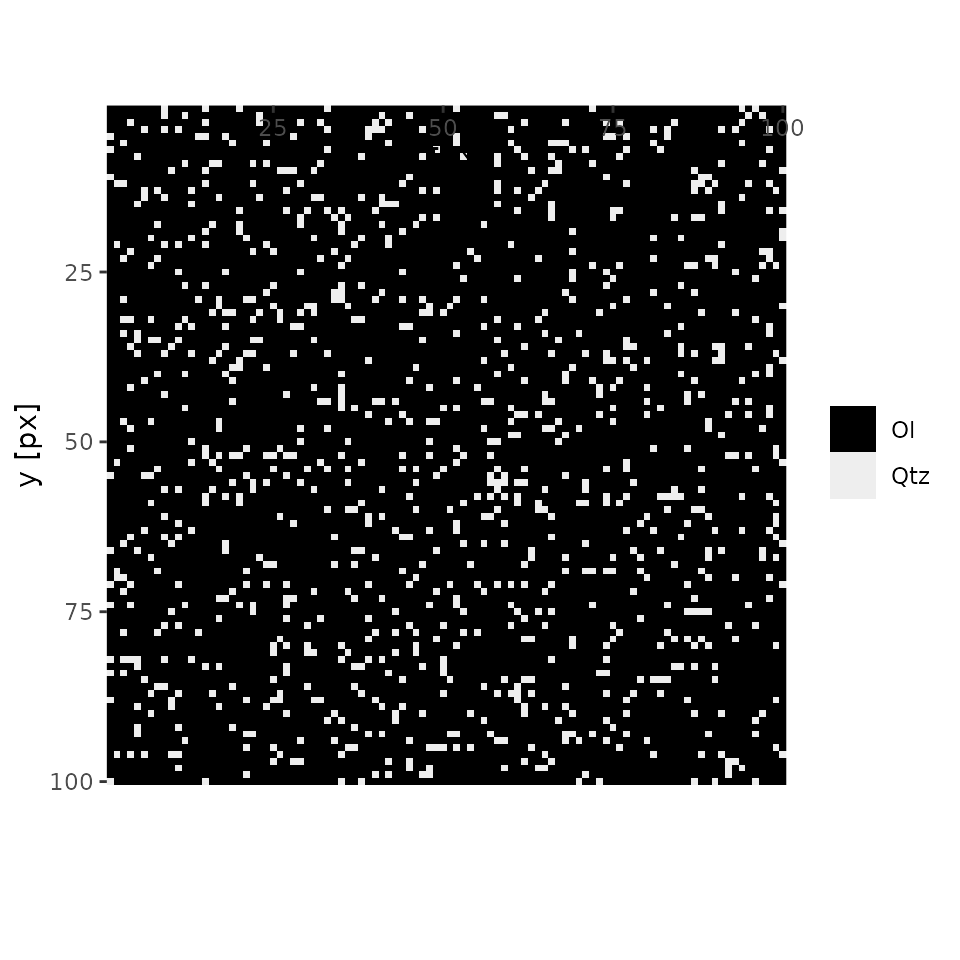
Quantify
qmap <- quantify(xmap = xmap, qnt = qnt, cluster = cluster)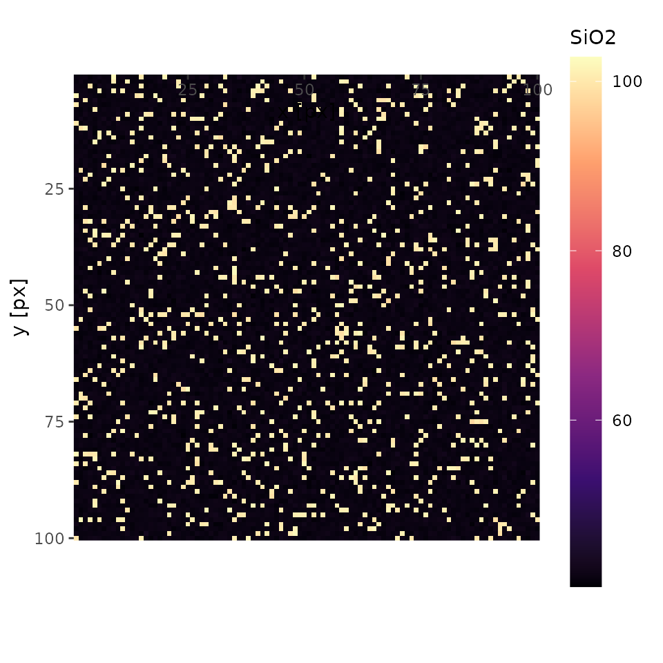
Summarize quantified map
summary(qmap)
#>   Element  Min. 1st Qu. Median  Mean 3rd Qu.   Max.
#> 1    SiO2 40.39   42.32  42.80 48.43   43.35 102.81
#> 2     MgO  0.00   56.46  57.10 51.49   57.68  59.87
#> 3   Total 96.28   99.23  99.94 99.92  100.61 104.20
Note also that this summary does not correct densities of phases.
According to compositions of olivine (57.29% MgO and 42.71 wt% SiO2), and of quartz (100% SiO2),
\[ E(MgO^{\mathrm{bulk}}) = 57.29 \times 0.9 + 0 \times 0.1 = 51.561 \simeq 51.49 \mathrm{,} \]
and
\[ E(SiO^{\mathrm{bulk}}_{2}) = 42.71 \times 0.9 + 100 \times 0.1 = 48.439 \simeq 48.43 \mathrm{,} \]
which are concordant to the above summary.
Summary based on mask images
A simple use of mean() function returns mean() values of each elements.
mean(qmap)
#>   Element Whole area
#> 1    SiO2   48.43475
#> 2     MgO   51.48943
#> 3   Total   99.92419
Further, by using PNG format mask image width and height are same as mapping data, mean() values of each element are calculated for each area with same colors in the mask image.
Let’s use an image from cluster analysis above.
Input path to the image to segment function.
Then, input the result of segment() to index parameter of mean().
mean(qmap, index = i)
#>   Element  #000000  #EEEEEE
#> 1    SiO2 42.71444 99.91753
#> 2     MgO 57.21048  0.00000
#> 3   Total 99.92492 99.91753
Alternatively, index parameter can be given as a character vector such as name of phases (i.e. . Thus, giving index = cluster$cluster returns a prettier result than the above.
mean(qmap, index = cluster$cluster)
#>   Element       Ol      Qtz
#> 1    SiO2 42.71444 99.91753
#> 2     MgO 57.21048  0.00000
#> 3   Total 99.92492 99.91753
The above two mean() values are equivalent as black (#000000) corresponds to olivine cluster, and white (#FFFFFF) to quartz cluster.
This feature is useful to find average compositions of each minearls, local bulk compositions of domains (layer, symplectite), and so on.